A complete multilevel ERGM analysis#
A multilevel network has vertices at two levels, such as researchers and the
laboratories they belong to, with ties within each level and affiliation
ties between them (Lazega et al. 2008). This page fits the multilevel ERGMs
of Wang, Robins, Pattison and Lazega (2013), as their program MPNet does,
to a network simulated from a known model, so we can check that the
estimates recover the true values. It draws the network with
multinets, then
describes, fits, checks, compares and reports the models with ergmx.
The data#
labs_sim has 120 researchers and 30 laboratories. Its vertex attribute
type is multinets’ convention for the levels (True for laboratories),
and level names them, for ergmx’s formulas. nodemix counts the ties
of each kind:
import random

import igraph as ig
import matplotlib.pyplot as plt
import multinets as mn

import ergmx
from ergmx import datasets

labs = datasets.load("labs_sim")  # an igraph.Graph
ergmx.summary_stats(labs, "nodemix('level', levels2=TRUE)")
{'mix.level.laboratory.laboratory': 61.0,
 'mix.level.laboratory.researcher': 150.0,
 'mix.level.researcher.researcher': 372.0}
The 120 researchers have 372 ties among them, and the 30 laboratories 61. The 150 affiliations are memberships: every researcher belongs to a laboratory, and a quarter of them to two.
Drawing the network#
multinets lays out each level on its own band, the laboratories above the researchers, and colours and shapes the vertices and ties by level:
random.seed(1)  # igraph's layouts use Python's random numbers
layout = mn.layout_multilevel(labs, layout="kk")
styled = mn.set_shape_multilevel(mn.set_color_multilevel(labs))

fig, ax = plt.subplots(figsize=(8, 7))
ig.plot(styled, target=ax, layout=layout, vertex_size=7, edge_width=0.6);
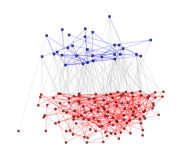
The laboratories are the blue squares, the researchers the red circles, and the affiliations the grey ties between them.
The model behind the data#
The memberships were drawn first. Then the ties within each level were simulated given them (the script), from a model with these effects:
Term |
Effect |
True value |
|---|---|---|
|
the researchers’ baseline log-odds of a tie |
-3.6 |
|
triadic closure among researchers |
0.3 |
|
the laboratories’ baseline log-odds of a tie |
-2.8 |
|
researchers of the same laboratory are tied |
1.5 |
|
laboratories that share a researcher are tied |
1.5 |
|
members of tied laboratories are tied: the levels are aligned |
0.4 |
The operator S() evaluates terms on the network within a set
of vertices (Multilevel networks). The last three terms
are MPNet’s configurations that join ties of different kinds. Their first
argument is the level attribute; its values in sorted order are level A,
the laboratories, and level B, the researchers. So txbx counts the ties
between researchers who share a laboratory, and txax those between
laboratories that share a researcher. c4axb counts the four-cycles of a
tie between researchers, a tie between laboratories and the two
affiliations that join them.
As the memberships are given, the models are fitted given them, with the
constraint blocks('level', levels2=2). It fixes the dyads of the second
mixing type, in nodemix’s order: (laboratory, laboratory), (laboratory,
researcher), (researcher, researcher) (Constraints).
A model of each level#
A first model has each level’s density and the closure among researchers, but nothing that joins the levels:
given = "blocks('level', levels2=2)"
levels = (
    "S(~edges + gwesp(0.693147, fixed=TRUE), ~level == 'researcher')"
    " + S(~edges, ~level == 'laboratory')"
)
separate = ergmx.ergm(labs, levels, constraints=given, seed=1)
separate.summary()
Monte Carlo Maximum Likelihood Results:

                                              Estimate  Std. Error  MCMC %  z value  Pr(>|z|)
S(level=="researcher")~edges                   -3.3490      0.0843       0  -39.714    <1e-04 ***
S(level=="researcher")~gwesp.fixed.0.693147     0.3924      0.0544       0    7.210    <1e-04 ***
S(level=="laboratory")~edges                   -1.8099      0.1392       0  -13.001    <1e-04 ***
---
Signif. codes:  0 '***' 0.001 '**' 0.01 '*' 0.05 '.' 0.1 ' ' 1

Log-likelihood: -1612.3163 (MC SE 0.091)   AIC: 3230.6327   BIC: 3251.4305
Constraints: blocks('level', levels2=2).
Converged after 3 iterations (4 chains, 1024 samples).
It overestimates the closure among researchers (0.39, against a true 0.3):
without the cross-level terms, the model takes the ties among members of
the same laboratory, who often share partners, for triadic closure. The
laboratories’ edges coefficient is their overall log-odds of a tie, far
above the baseline of the true model.
Adding the cross-level effects#
cross = " + txbx('level') + txax('level') + c4axb('level')"
multilevel = ergmx.ergm(labs, levels + cross, constraints=given, seed=1, interval=4096)
multilevel.summary()
Monte Carlo Maximum Likelihood Results:

                                              Estimate  Std. Error  MCMC %  z value  Pr(>|z|)
S(level=="researcher")~edges                   -3.5916      0.0848       0  -42.331    <1e-04 ***
S(level=="researcher")~gwesp.fixed.0.693147     0.3107      0.0536       0    5.795    <1e-04 ***
S(level=="laboratory")~edges                   -2.7980      0.2091       0  -13.379    <1e-04 ***
TXBX.level                                      1.5367      0.1301       0   11.808    <1e-04 ***
TXAX.level                                      1.7962      0.4305       0    4.172    <1e-04 ***
C4AXB.level                                     0.4471      0.0629       0    7.108    <1e-04 ***
---
Signif. codes:  0 '***' 0.001 '**' 0.01 '*' 0.05 '.' 0.1 ' ' 1

Log-likelihood: -1510.1644 (MC SE 0.190)   AIC: 3032.3287   BIC: 3073.9244
Constraints: blocks('level', levels2=2).
Converged after 3 iterations (4 chains, 1024 samples).
interval=4096 spaces the networks of the MCMC sample by 4096 proposals,
four times the default, for better mixing (see the next section). Sharing
a laboratory multiplies the odds of a tie between two researchers by about
exp(1.54) = 4.7, and sharing a researcher those of two laboratories by
about exp(1.80) = 6.
Are the true values recovered?#
truth = {
    'S(level=="researcher")~edges': -3.6,
    'S(level=="researcher")~gwesp.fixed.0.693147': 0.3,
    'S(level=="laboratory")~edges': -2.8,
    "TXBX.level": 1.5,
    "TXAX.level": 1.5,
    "C4AXB.level": 0.4,
}
intervals = multilevel.confint().to_dict()
print(f"{'':<45}{'true':>6}{'estimate':>10}   95% interval")
for name, value in truth.items():
    low, high = intervals[name].values()
    print(f"{name:<45}{value:>6.1f}{multilevel.coef[name]:>10.2f}   [{low:.2f}, {high:.2f}]")
                                               true  estimate   95% interval
S(level=="researcher")~edges                   -3.6     -3.59   [-3.76, -3.43]
S(level=="researcher")~gwesp.fixed.0.693147     0.3      0.31   [0.21, 0.42]
S(level=="laboratory")~edges                   -2.8     -2.80   [-3.21, -2.39]
TXBX.level                                      1.5      1.54   [1.28, 1.79]
TXAX.level                                      1.5      1.80   [0.95, 2.64]
C4AXB.level                                     0.4      0.45   [0.32, 0.57]
Every true value is inside its 95% interval.
Did the estimation converge?#
As for any Monte Carlo MLE, the simulated networks should reproduce the observed statistics, and the chains agree and be stationary (Convergence and MCMC diagnostics):
multilevel.mcmc_diagnostics()
MCMC diagnostics of the last iteration: 4 chains x 1024 samples, 4096 proposals apart

Sample statistics, as deviations from the observed statistics:

                                                  Mean         SD   Naive SE  Time-series SE  Eff. size   R-hat
S(level=="researcher")~edges                    -0.552     27.095     0.4234          0.6415       1784   1.002
S(level=="researcher")~gwesp.fixed.0.693147      0.368     44.194     0.6905          1.0398       1806   1.002
S(level=="laboratory")~edges                     0.477      7.003     0.1094          0.1623       1863   1.002
TXBX.level                                      -0.447      9.724     0.1519          0.2283       1814   1.000
TXAX.level                                       0.052      2.653     0.0415          0.0608       1906   1.003
C4AXB.level                                      1.505     31.507     0.4923          0.8600       1342   1.002

Are the sample statistics significantly different from the observed?
Hotelling's T^2 test p-value: 0.0005. The largest mean deviation is 0.068 SD; with large effective sizes, even negligible deviations are significant.

Geweke z-scores (first 10% against last 50% of each chain):

                                              chain 1   chain 2   chain 3   chain 4
S(level=="researcher")~edges                    -0.61     -0.19      1.15     -0.01
S(level=="researcher")~gwesp.fixed.0.693147     -0.90     -0.05      0.61      0.26
S(level=="laboratory")~edges                    -0.59      0.07      0.88     -0.98
TXBX.level                                      -0.29      0.32      0.73      0.03
TXAX.level                                      -0.88     -0.86     -0.18     -1.35
C4AXB.level                                     -1.26     -0.40      0.63     -0.53

0 of 24 Geweke z-scores have p < 0.05 (about 1.2 expected by chance).
The mean deviations are below a tenth of an SD, R-hat is close to 1, and no Geweke z-score is beyond ±2. Hotelling’s test flags the deviations as significant only because the effective sizes are large: they are negligible. With the default interval of 1024 proposals, 4 of the 24 Geweke z-scores were beyond ±2: the chains hadn’t mixed as well.
Does the model fit each level?#
gof() with by="level" compares each level’s network
with those of 100 networks simulated from the model (given the memberships,
as the fit): its degrees, edgewise shared partners and distances, as MPNet’s
goodness of fit does (Goodness of fit):
multilevel.gof(by="level", stats=["degree", "espartners", "distance"], seed=1).plot();
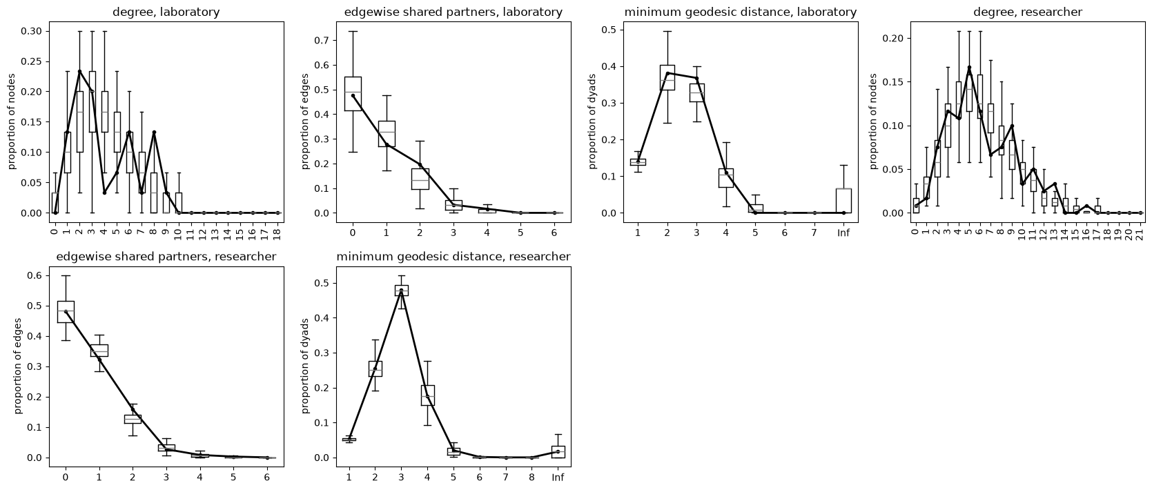
The model reproduces both levels’ distributions (the black lines are the observed ones, the boxplots the simulated ones), as the true model should. The laboratories’ degrees are noisier, as there are only 30 of them: one laboratory with 4 ties and four with 8 are at the edge of the simulations, deviations that happen by chance with so few vertices.
Which model is better?#
ergmx.compare(separate, multilevel)
Model comparison:

      df        log-likelihood         AIC         BIC     dAIC   LR chi2   df  Pr(>chi2)
  1    3     -1612.316 (0.091)     3230.63     3251.43   198.30
  2    6     -1510.164 (0.190)     3032.33     3073.92     0.00    204.30    3  4.956e-44

  1: S(edges() + gwesp(0.693147, fixed=True), "~level == 'researcher'") + S(edges(), "~level == 'laboratory'")
  2: S(edges() + gwesp(0.693147, fixed=True), "~level == 'researcher'") + S(edges(), "~level == 'laboratory'") + txbx('level') + txax('level') + c4axb('level')

Log-likelihoods of dyad-dependent models are Monte Carlo estimates (standard errors in parentheses).
The cross-level effects improve the model enormously: the AIC is about 200 lower, and the likelihood-ratio test is highly significant. The levels are not independent: who collaborates with whom among researchers depends on their laboratories, and the other way round.
Reporting the results#
ergmx.table() puts the models side by side, with rename= for
readable labels:
ergmx.table(
    separate,
    multilevel,
    names=["Each level", "Multilevel"],
    rename={
        'S(level=="researcher")~edges': "Researchers: edges",
        'S(level=="researcher")~gwesp.fixed.0.693147': "Researchers: GWESP",
        'S(level=="laboratory")~edges': "Laboratories: edges",
        "TXBX.level": "Same laboratory (TXBX)",
        "TXAX.level": "Shared researcher (TXAX)",
        "C4AXB.level": "Alignment (C4AXB)",
    },
)
| Each level | Multilevel | |
|---|---|---|
| Researchers: edges | -3.35*** | -3.59*** |
| (0.08) | (0.08) | |
| Researchers: GWESP | 0.39*** | 0.31*** |
| (0.05) | (0.05) | |
| Laboratories: edges | -1.81*** | -2.80*** |
| (0.14) | (0.21) | |
| Same laboratory (TXBX) | 1.54*** | |
| (0.13) | ||
| Shared researcher (TXAX) | 1.80*** | |
| (0.43) | ||
| Alignment (C4AXB) | 0.45*** | |
| (0.06) | ||
| AIC | 3230.63 | 3032.33 |
| BIC | 3251.43 | 3073.92 |
| Log Likelihood | -1612.32 | -1510.16 |
| ***p < 0.001; **p < 0.01; *p < 0.05 | ||
Multilevel networks has every MPNet configuration, how
each MPNet effect is written in ergmx, and other ways to model multilevel
networks.