Samples of networks

Many studies observe not one network but many: the friendships in each classroom of a school, the contacts within each household of a survey, the advice networks of several firms. Fitting one ERGM per network gives as many estimates as networks, each noisy if the networks are small. Fitting a single model to all of them, as R’s ergm.multi does (Krivitsky, Coletti and Hens 2023), pools their information, and can let the effects depend on each network’s characteristics.

The Goeyvaerts data (Goeyvaerts et al. 2018), from ergm.multi, are the contacts within 318 households of Flanders and Brussels, each from a one-day contact diary:

import ergmx
from ergmx import datasets

households = datasets.load("Goeyvaerts")   # a list of igraph.Graph
print(datasets.describe("Goeyvaerts"))
households[0].vs["role"], households[0]["weekday"]

A list of 318 networks: the contacts within households with at least one child aged 12 or under, in Flanders and Brussels, from contact diaries (Goeyvaerts et al. 2018, Proc. R. Soc. B 285: 20182201, doi:10.1098/rspb.2018.2201; curated by Pietro Coletti for R's ergm.multi; cite both when publishing). Undirected. Vertex attributes: age, gender ('F', 'M') and role ('Father', 'Mother', 'Child', 'Grandmother'). Graph attributes: weekday (whether the diary was kept on a weekday) and included (whether Goeyvaerts et al. analysed it; two were not).

(['Father', 'Mother', 'Child', 'Child', 'Child'], True)

Each network has vertex attributes (age, gender, role) and graph attributes (weekday, whether the diary was kept on a weekday; included, whether the original study analysed it). Following the study, we keep the included households observed on a weekday:

weekday = [g for g in households if g["included"] and g["weekday"]]
len(weekday)

225

Networks() and N()

ergmx.Networks() combines networks for a joint model, and the operator N() evaluates terms on each network, as in ergm.multi. With N(~edges + triangle), the statistics are the sums over the households of their edges and triangles, so each coefficient is the same in every household:

networks = ergmx.Networks(weekday)
ergmx.summary_stats(networks, "N(~edges + triangle)")

{'N(1)~edges': 1300.0, 'N(1)~triangle': 934.0}

The networks are the blocks of one larger network, with no ties possible between them: each household’s model is the same ERGM, and the households are independent. Terms outside N() are evaluated on that combined network, as in ergm.multi; for most terms (edges, triangle, nodematch…) that is the same as summing them, but not for terms that count pairs of vertices, such as dsp, which would count the pairs in different households too.

Effects that depend on the network

N()’s second argument, lm, is a linear model for the coefficients, in R’s lm() syntax, over network-level attributes: each network’s graph attributes, n (its number of vertices), .NetworkID (1, 2…) and .NetworkName. N(~edges, ~I(n <= 3) + I(n >= 5)) has three parameters: the edges coefficient of medium households (3 to 4 members, the intercept), and how much higher it is in small and in large ones. This is the model of ergm.multi’s vignette, with the terms ergmx has:

formula = (
    "N(~edges, ~I(n <= 3) + I(n >= 5)) "
    "+ N(~kstar(2) + nodematch('gender') + absdiff('age')) "
    "+ N(~triangle, ~I(n >= 6))"
)
fit = ergmx.ergm(networks, formula, seed=1)
fit.summary()

Monte Carlo Maximum Likelihood Results:

                            Estimate  Std. Error  MCMC %  z value  Pr(>|z|)
N(1)~edges                    0.2651      0.4838       0    0.548   0.58371 
N(I(n <= 3)TRUE)~edges        1.4078      0.4552       0    3.093   0.00198 **
N(I(n >= 5)TRUE)~edges       -0.7492      0.2321       0   -3.227   0.00125 **
N(1)~kstar2                  -0.5458      0.2416       0   -2.259   0.02387 *
N(1)~nodematch.gender        -0.2159      0.2142       0   -1.008   0.31335 
N(1)~absdiff.age              0.0335      0.0089       0    3.758   0.00017 ***
N(1)~triangle                 2.4074      0.3285       0    7.329    <1e-04 ***
N(I(n >= 6)TRUE)~triangle    -0.3390      0.1101       0   -3.079   0.00208 **
---
Signif. codes:  0 '***' 0.001 '**' 0.01 '*' 0.05 '.' 0.1 ' ' 1

Log-likelihood: -327.2852 (MC SE 0.180)   AIC: 670.5703   BIC: 712.6657
Fitted to 225 networks.
Converged after 6 iterations (4 chains, 1024 samples).

Contacts are denser in small households and sparser in large ones. They close triangles strongly: two members in contact with a third tend to be in contact with each other, less so in the largest households. And they are more likely between members of different ages (parents and children) than the rest of the model predicts. R’s ergm.multi gives the same estimates, in about eight times as long (see Validation).

The names follow ergm.multi: N(1)~edges for the intercept, then each column of the linear model, named as R’s model.matrix() names it, such as N(I(n <= 3)TRUE)~edges for a logical term or N(log(n))~edges for a numeric one. Factors and character attributes get one column per level but the first; ~0 + factor(.NetworkID) gives each network its own coefficient.

The lm formula accepts attributes, arithmetic, comparisons, &, |, !, I(), log(), exp(), sqrt(), abs(), factor() and offset(); interactions (a:b) are not supported yet.

N()’s other arguments are ergm.multi’s. subset restricts the terms to some networks, an expression of their attributes such as ~n >= 4 (or logical values, or indices): the others contribute nothing, and the linear model’s levels are those of the networks kept. offset adds a known amount to every coefficient of the formula in each network, such as ~log(n): the statistics get companions offset1, offset2…, whose coefficients are fixed at 1. label names the operator in the statistics’ names, N(<label>,1)~edges, which tells apart the parameters of several N() terms:

ergmx.summary_stats(networks, "N(~edges, subset=~n >= 4, label='big') + N(~edges, offset=~log(n))")

{'N(big,1)~edges': 1138.0, 'N(1)~edges': 1300.0, 'offset1': 1901.73301132092}

Curved terms

A curved term inside N(), such as gwesp(0.5), has parameters that the linear model predicts for each network, like any term’s: N(~edges + gwesp(0.5), ~log(n)) estimates how the gwesp coefficient and its decay change with the network size. Because a curved term’s statistics enter the likelihood nonlinearly in its parameters, its statistics can’t be summed over the networks: the model keeps each network’s histogram counts instead, named N#1~esp#1, N#1~esp#2… as in ergm.multi.

Checking and using the fit

Everything else works as for one network: mcmc_diagnostics(), ergmx.compare(), the log-likelihood (summed over the networks) and BIC (with the number of dyads within networks). gof() compares the distributions summed over the networks:

fit.gof(seed=1, stats=["degree", "espartners", "model"]).plot();

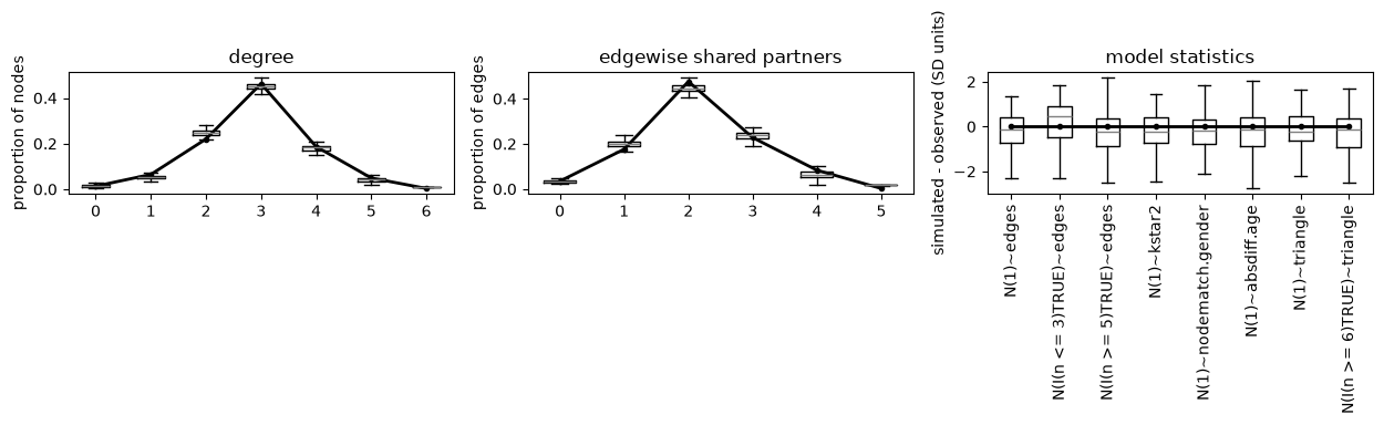
Distances and shared partners only count pairs of vertices in the same network; ergm’s gof() also counts the pairs in different networks, as unreachable. simulate() returns, for each simulation, a list with one network per household:

first = fit.simulate(1, seed=1)[0]
len(first), [g.ecount() for g in first[:5]], [g.ecount() for g in weekday[:5]]

(225, [10, 6, 3, 6, 6], [10, 6, 3, 3, 6])

Goodness of fit network by network

Summed distributions can hide a model that fits some networks and not others. ergmx.gofN(), as ergm.multi’s gofN(), compares each network’s statistics with those simulated from the fit: their mean (the fitted value), variance, and the Pearson residual, (observed - fitted) / sd. By default the statistics are the model’s, each network’s share; GOF= checks others. Its summary describes the residuals over the networks, whose variance is near 1 for a model that fits:

by_household = ergmx.gofN(fit, "edges + triangle + kstar(2)", seed=1)
by_household.summary()

Observed/Imputed values
              Min.   1st Qu.    Median      Mean   3rd Qu.      Max.      NA's
edges            1         3         6     5.778         6        18         0
triangle         0         1         4     4.324         4        23         9
kstar2           0         3        12     13.55        12        78         9

Fitted values
              Min.   1st Qu.    Median      Mean   3rd Qu.      Max.      NA's
edges         0.86      2.95      5.58     5.751      5.79     20.88         0
triangle      0.84     2.855      3.38     4.266     3.685      34.4         9
kstar2        2.66     9.308     10.59     13.39     11.31     103.8         9

Pearson residuals
              Min.   1st Qu.    Median      Mean   3rd Qu.      Max.      NA's
edges       -8.818    0.2031    0.3867  -0.08683    0.4984      1.32         0
triangle    -6.981    0.2031    0.4473  -0.04122    0.5761     1.658         9
kstar2        -7.9    0.2031    0.4241  -0.06692    0.5414     1.508         9

Variance and std. dev. of the Pearson residuals
edges        1.779     1.334
triangle     1.456     1.207
kstar2       1.618     1.272

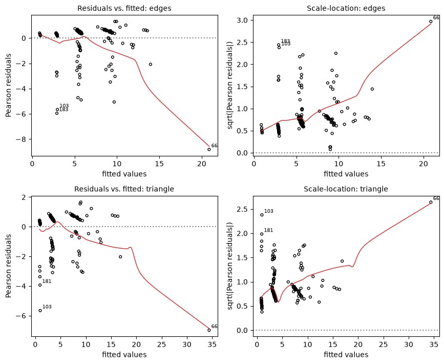
Indexing by statistic gives the table of the networks (.to_frame() as a pandas DataFrame), and plot() the residuals against the fitted values (or against=, an expression of the networks’ attributes) and their scale-location plot, with a weighted local regression to show a trend and the most extreme networks labelled:

by_household.plot(["edges", "triangle"]);

summary(by=) splits the summary by an attribute of the networks, such as by="~n", and subset= keeps some networks. With missing dyads, the observed statistics are averaged over networks imputed from the model, as in ergm.multi.

ergm.multi’s gofN() leaves out the statistics of the empty network, so it reports degree0 and isolates minus the network size; ergmx reports the statistics themselves, and warns (ErgmDifferenceWarning) when the statistics checked have this difference. Its default interval between simulated networks is three times the number of dyads, where ergm.multi uses the fit’s (1024 by default): with many small networks, each network’s simulated statistics are then autocorrelated, and its fitted values and residuals about twice as noisy as nsim independent draws.