A complete ERGM analysis#
This page takes a friendship network from the data to a table of results: describe it, fit a model, check that the estimation converged and that the model fits, compare it with a simpler model, interpret it and report it.
The data#
faux.mesa.high is a friendship network of 205 students of a high school,
simulated from the Add Health study design, with each student’s grade, race
and sex:
import random

import igraph as ig
import matplotlib.pyplot as plt

import ergmx
from ergmx import datasets

mesa = datasets.load("faux.mesa.high")  # an igraph.Graph
print(f"{mesa.vcount()} students, {mesa.ecount()} friendships, density {mesa.density():.4f}")
print(f"{len(mesa.vs.select(_degree=0))} students have no friends in the school")
205 students, 203 friendships, density 0.0097
57 students have no friends in the school
Drawn with igraph, each student coloured by grade:
random.seed(1)  # igraph's layouts use Python's random numbers
grades = sorted(set(mesa.vs["Grade"]))
colors = plt.get_cmap("viridis", len(grades))

fig, ax = plt.subplots(figsize=(8, 7))
ig.plot(
    mesa, target=ax, layout=mesa.layout("fr"), vertex_size=6, edge_width=0.4, edge_color="grey",
    vertex_color=[colors(grades.index(g)) for g in mesa.vs["Grade"]],
)
ax.legend(
    handles=[plt.Line2D([], [], marker="o", linestyle="", color=colors(k), label=f"Grade {g:g}")
             for k, g in enumerate(grades)],
    loc="upper left", bbox_to_anchor=(1, 1), frameon=False,
);
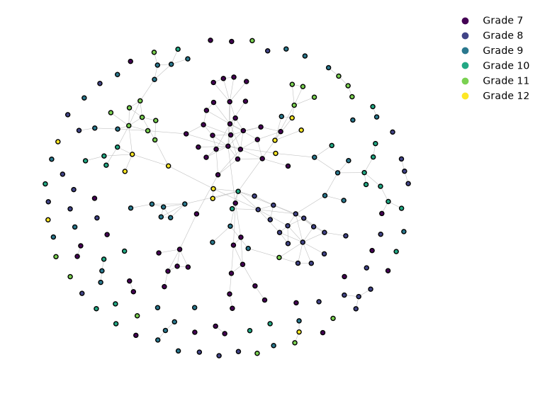
Friends tend to be in the same grade, and they form clusters. Before
modelling, ergmx.summary_stats() counts the statistics a model could
use, as R’s summary(formula)
(Formulas, Term reference):
ergmx.summary_stats(mesa, "edges + nodematch('Grade') + nodematch('Race') + nodematch('Sex') + triangle")
{'edges': 203.0,
 'nodematch.Grade': 163.0,
 'nodematch.Race': 103.0,
 'nodematch.Sex': 132.0,
 'triangle': 62.0}
Of the 203 friendships, 163 are between students of the same grade, and there are 62 triangles of friends.
A first model: homophily#
ergmx.ergm() fits a model given as an R-style formula. The first one
has the baseline log-odds of a friendship (edges), a difference between
boys and girls in their number of friendships (nodefactor('Sex')), and
homophily on grade and race (nodematch):
homophily = ergmx.ergm(mesa, "edges + nodefactor('Sex') + nodematch('Grade') + nodematch('Race')")
homophily.summary()
Maximum Likelihood Results:

                   Estimate  Std. Error  MCMC %  z value  Pr(>|z|)
edges               -5.8917      0.1953       0  -30.169    <1e-04 ***
nodefactor.Sex.M    -0.3481      0.1024       0   -3.398   0.00068 ***
nodematch.Grade      2.8150      0.1774       0   15.864    <1e-04 ***
nodematch.Race       0.4262      0.1429       0    2.982   0.00286 **
---
Signif. codes:  0 '***' 0.001 '**' 0.01 '*' 0.05 '.' 0.1 ' ' 1

Log-likelihood: -959.4767   AIC: 1926.9533   BIC: 1958.7453
Students of the same grade are much more likely to be friends, and so, less, are students of the same race; boys have fewer friendships than girls. These terms are dyad-independent: each friendship is independent of the others, so the estimates are a logistic regression’s, exact (Fitting models).
Adding triadic closure#
Friendships are not independent, though: friends of friends become friends.
gwesp, the geometrically weighted edgewise shared partners, counts the
friendships whose two students share friends, with less weight on each
further shared friend:
closure = ergmx.ergm(
    mesa,
    "edges + nodefactor('Sex') + nodematch('Grade') + nodematch('Race') + gwesp(0.5, fixed=TRUE)",
    seed=1,
)
closure.summary()
Monte Carlo Maximum Likelihood Results:

                   Estimate  Std. Error  MCMC %  z value  Pr(>|z|)
edges               -6.1846      0.1734       0  -35.669    <1e-04 ***
nodefactor.Sex.M    -0.1256      0.0747       0   -1.681   0.09274 .
nodematch.Grade      1.9710      0.1758       0   11.210    <1e-04 ***
nodematch.Race       0.2657      0.1188       0    2.235   0.02539 *
gwesp.fixed.0.5      1.2166      0.0853       0   14.271    <1e-04 ***
---
Signif. codes:  0 '***' 0.001 '**' 0.01 '*' 0.05 '.' 0.1 ' ' 1

Log-likelihood: -867.1531 (MC SE 0.194)   AIC: 1744.3062   BIC: 1784.0461
Converged after 6 iterations (4 chains, 1024 samples).
Triadic closure is strong (gwesp), and with it in the model the effect of
grade is smaller: part of what looked like homophily was friends of friends,
who are often in the same grade. The difference between boys and girls is
no longer significant. The model is dyad-dependent, so it is fitted by Monte
Carlo maximum likelihood, from networks simulated by MCMC; seed= makes
the result reproducible.
Did the estimation converge?#
At the estimate, the networks simulated from the model should have the observed statistics on average, and the MCMC chains should agree (Convergence and MCMC diagnostics):
diagnostics = closure.mcmc_diagnostics()
diagnostics
MCMC diagnostics of the last iteration: 4 chains x 1024 samples, 4096 proposals apart

Sample statistics, as deviations from the observed statistics:

                       Mean         SD   Naive SE  Time-series SE  Eff. size   R-hat
edges                 0.766     39.342     0.6147          1.9556        405   1.006
nodefactor.Sex.M      0.552     31.783     0.4966          1.3877        525   1.005
nodematch.Grade       0.940     37.965     0.5932          1.9041        398   1.006
nodematch.Race        0.221     23.219     0.3628          1.1181        431   1.007
gwesp.fixed.0.5       1.134     57.164     0.8932          2.8675        397   1.007

Are the sample statistics significantly different from the observed?
Hotelling's T^2 test p-value: 0.9748. The largest mean deviation is 0.025 SD; with large effective sizes, even negligible deviations are significant.

Geweke z-scores (first 10% against last 50% of each chain):

                   chain 1   chain 2   chain 3   chain 4
edges                -0.00      1.53      0.39      1.22
nodefactor.Sex.M      0.14      2.44      0.03      1.23
nodematch.Grade      -0.13      1.41      0.37      1.23
nodematch.Race       -0.15      1.66      0.38      1.05
gwesp.fixed.0.5      -0.08      1.42      0.43      1.15

1 of 20 Geweke z-scores have p < 0.05 (about 1.0 expected by chance).
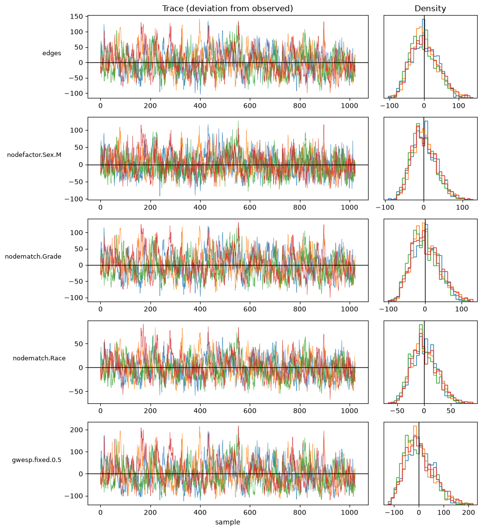
The mean deviations are a small fraction of the SDs, the four chains agree (R-hat close to 1), and the samples are worth hundreds of independent ones (the effective sizes). The traces should look like noise around zero, and the chains’ densities overlap:
diagnostics.plot();
Does the model fit?#
Each model reproduces the statistics in its formula, but does it reproduce
the rest of the network’s structure? gof() simulates
100 networks from the model and compares their degree, edgewise shared
partner and geodesic distance distributions with the observed network’s
(Goodness of fit). The black lines are the observed
distributions and the boxplots the simulated ones, here for each model:
stats = ["degree", "espartners", "distance"]
fig, axes = plt.subplots(2, 3, figsize=(13, 7))
homophily.gof(stats=stats, seed=1).plot(axes[0])
closure.gof(stats=stats, seed=1).plot(axes[1])
for model, row in zip(["Homophily", "Closure"], axes):
    for ax in row:
        ax.set_title(f"{model}: {ax.get_title()}")
fig.tight_layout()
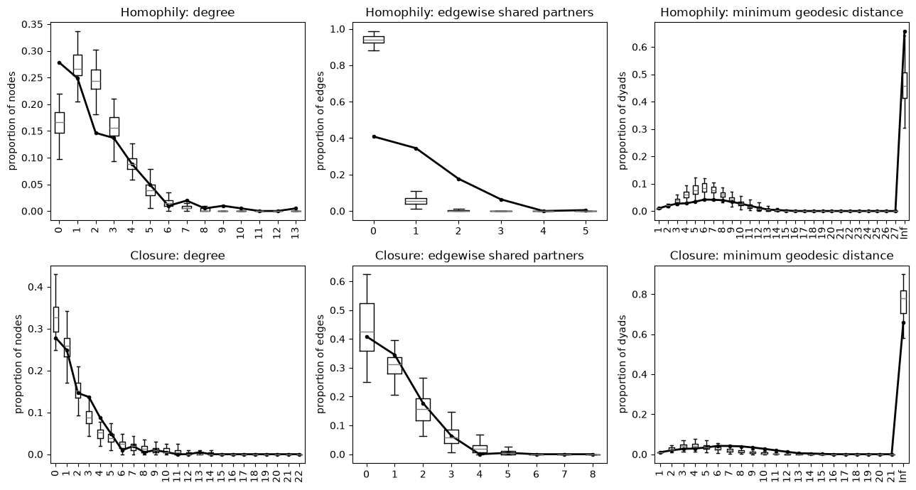
The homophily model misses the shared partners: in its networks, almost no two friends share a friend. Its networks are also too connected, with fewer students without friends, and fewer pairs of students who can’t reach each other, than the school. The closure model reproduces the shared partners and, roughly, the degrees. The school still has more pairs of students 8 to 12 steps apart than its networks: it is made of longer chains of friendships.
Which model is better?#
ergmx.compare() puts the models side by side, with their AIC and BIC
and, as they are nested, a likelihood-ratio test
(Model comparison):
ergmx.compare(homophily, closure)
Model comparison:

      df        log-likelihood         AIC         BIC     dAIC   LR chi2   df  Pr(>chi2)
  1    4              -959.477     1926.95     1958.75   182.65
  2    5      -867.153 (0.194)     1744.31     1784.05     0.00    184.65    1  4.686e-42

  1: edges() + nodefactor('Sex') + nodematch('Grade') + nodematch('Race')
  2: edges() + nodefactor('Sex') + nodematch('Grade') + nodematch('Race') + gwesp(0.5, fixed=True)

Log-likelihoods of dyad-dependent models are Monte Carlo estimates (standard errors in parentheses).
Adding triadic closure lowers the AIC by 183, far more than the Monte Carlo error of the log-likelihood.
Interpreting the coefficients#
A coefficient is the change in the log-odds of a friendship, given the rest of the network, for each unit of its statistic. Its exponential is an odds ratio (Interpreting and reporting results):
closure.odds_ratios()
Odds ratios, with 95% confidence intervals:

                  Odds ratio   2.5 %   97.5 %
edges                 0.0021  0.0015   0.0029
nodefactor.Sex.M      0.8820  0.7619   1.0210
nodematch.Grade       7.1781  5.0857  10.1314
nodematch.Race        1.3043  1.0333   1.6464
gwesp.fixed.0.5       3.3757  2.8562   3.9896

The factor by which a unit increase in the term's statistic multiplies the conditional odds of a tie.
Students of the same grade have about 7 times the odds of a friendship of others with the same friends, race and sex, and those of the same race 1.3 times. A first shared friend multiplies the odds by about 3.4. The same page has tie probabilities and marginal effects.
Reporting the results#
ergmx.table() puts the models side by side for a paper, as R’s texreg,
with rename= for readable labels:
results = ergmx.table(
    homophily,
    closure,
    names=["Homophily", "Closure"],
    rename={
        "edges": "Edges",
        "nodefactor.Sex.M": "Male",
        "nodematch.Grade": "Same grade",
        "nodematch.Race": "Same race",
        "gwesp.fixed.0.5": "GWESP (decay 0.5)",
    },
)
results
| Homophily | Closure | |
|---|---|---|
| Edges | -5.89*** | -6.18*** |
| (0.20) | (0.17) | |
| Male | -0.35*** | -0.13 |
| (0.10) | (0.07) | |
| Same grade | 2.81*** | 1.97*** |
| (0.18) | (0.18) | |
| Same race | 0.43** | 0.27* |
| (0.14) | (0.12) | |
| GWESP (decay 0.5) | 1.22*** | |
| (0.09) | ||
| AIC | 1926.95 | 1744.31 |
| BIC | 1958.75 | 1784.05 |
| Log Likelihood | -959.48 | -867.15 |
| ***p < 0.001; **p < 0.01; *p < 0.05 | ||
print(results) gives the text table, and .to_latex(), .to_html() and
.to_markdown() the others:
with open("models.tex", "w") as f:
    f.write(results.to_latex())
Next, A complete multilevel ERGM analysis does the same for a network with two levels.