Convergence and MCMC diagnostics

A Monte Carlo MLE is only as good as its MCMC sample. At the estimate, networks simulated from the model should have, on average, the observed statistics, and the chains should have explored the same distribution. ErgmFit.mcmc_diagnostics() checks both on the sample of the last iteration, like R’s mcmc.diagnostics():

import ergmx
from ergmx import datasets

mesa = datasets.load("faux.mesa.high")
fit = ergmx.ergm(
    mesa, "edges + nodematch('Grade') + nodematch('Race') + gwesp(0.5, fixed=TRUE)", seed=1
)
diagnostics = fit.mcmc_diagnostics()
diagnostics

MCMC diagnostics of the last iteration: 4 chains x 1024 samples, 4096 proposals apart

Sample statistics, as deviations from the observed statistics:

                      Mean         SD   Naive SE  Time-series SE  Eff. size   R-hat
edges                2.383     43.541     0.6803          2.3834        334   1.007
nodematch.Grade      2.248     42.221     0.6597          2.3480        323   1.008
nodematch.Race       0.673     25.471     0.3980          1.3362        363   1.007
gwesp.fixed.0.5      3.623     63.273     0.9886          3.5360        320   1.008

Are the sample statistics significantly different from the observed?
Hotelling's T^2 test p-value: 0.5667. The largest mean deviation is 0.057 SD; with large effective sizes, even negligible deviations are significant.

Geweke z-scores (first 10% against last 50% of each chain):

                  chain 1   chain 2   chain 3   chain 4
edges               -1.63      0.01      1.43      1.35
nodematch.Grade     -1.58      0.02      1.54      1.34
nodematch.Race      -1.45     -0.04      1.28      1.41
gwesp.fixed.0.5     -1.59     -0.07      1.70      1.23

0 of 16 Geweke z-scores have p < 0.05 (about 0.8 expected by chance).

What to look for:

Mean deviations

Near zero, compared with the SD: the simulated networks reproduce the observed statistics. With thousands of effective samples, Hotelling’s test flags even negligible deviations, so look at their size too.

Effective size

How many independent samples the autocorrelated sample is worth. Small values (below a hundred or so) make the estimate and its standard errors noisy; raise interval or samplesize.

R-hat

Compares the parallel chains. Close to 1 means they agree; above 1.1, they are exploring different parts of the distribution, a sign of poor mixing or of a degenerate model.

Geweke z-scores

Compare the start and the end of each chain. About one in twenty beyond ±2 is expected by chance; many more suggest the chains had not reached their stationary distribution.

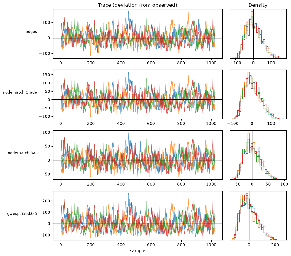
The plots show the same: traces should look like noise around zero, and the chains’ densities should overlap.

diagnostics.plot();

Degenerate models

Some models put almost all their probability on nearly empty or nearly complete networks: they are degenerate. No coefficients make their simulated networks look like the observed one, and the estimation can’t converge. ergmx detects this and stops with a ergmx.DegeneracyError that says why:

samplk3 = datasets.load("samplk3")

try:
    ergmx.ergm(samplk3, "edges + mutual", init=[4.0, 0.0], seed=1, stall_iterations=2)
except ergmx.DegeneracyError as error:
    print(error)

the Monte Carlo MLE is not making progress: for 2 iterations the observed statistics were far outside the range of the simulated networks (step lengths below 0.1). The model may be degenerate, or the starting coefficients poor.

At the current coefficients:
             simulated      observed
  edges          10.00         56.00
  mutual          4.99         15.00

Things to try: other terms (for example gwesp with a smaller decay instead of triangle), adding gwdegree or attribute terms, init='CD', or a longer MCMC (interval=...). Control(stall_iterations=None) keeps iterating.

Here the starting coefficients are just poor, which init="MPLE" (the default) avoids. Two checks raise the error:

• The density guard, as in ergm: a simulated network with many more edges than the observed one (Control.density_guard, by default about 20 times, and at least density_guard_min edges). The chains stop as soon as it trips, so it costs little time.

• A stalled estimation: stall_iterations consecutive iterations (10 by default) in which the observed statistics are far outside the range of the simulated ones. The time this takes depends on the model, as later iterations use longer chains. stall_iterations=None keeps iterating.

Degeneracy is usually fixed by changing the model rather than the settings: gwesp with a smaller decay instead of triangle, adding gwdegree or attribute terms, or a starting point closer to the MLE (init="CD").