Multilevel networks#
A multilevel network has vertices at several levels, such as researchers and
the laboratories they belong to, with ties within each level (advice among
researchers, collaboration among laboratories) and ties across levels (the
affiliations) (Lazega and Snijders 2016). In ergmx it is one network with a
vertex attribute for the level. Wang, Robins, Pattison and Lazega (2013)
proposed ERGMs for such two-level networks, as their program MPNet fits them:
a level A, a level B, the A-ties within A, the B-ties within B, and the X-ties
between them, with effects for each network and for how they depend on each
other.
linked_sim, from the multinets
package, has 100 individuals and 50 organizations:
import ergmx
from ergmx import datasets

linked = datasets.load("linked_sim")
ergmx.summary_stats(linked, "nodemix('level', levels2=TRUE)")
{'mix.level.individual.individual': 304.0,
 'mix.level.individual.organization': 207.0,
 'mix.level.organization.organization': 89.0}
Each level, and the ties between them#
The operator S(), as ergm’s, evaluates terms on a subgraph. With
one set of vertices, ~level == 'individual', it is the network within that
level, so any ergm term describes it; with two, (level == 'individual') ~ (level == 'organization'), it is the bipartite network of the ties between
them, whose b1 terms are about the first set:
ergmx.summary_stats(
    linked,
    "S(~edges + gwesp(0.693147, fixed=TRUE), ~level == 'individual') "
    "+ S(~edges + b1star(2) + b2star(2), (level == 'individual') ~ (level == 'organization'))",
)
{'S(level=="individual")~edges': 304.0,
 'S(level=="individual")~gwesp.fixed.0.693147': 102.1249985780903,
 'S((level=="individual"),(level=="organization"))~edges': 207.0,
 'S((level=="individual"),(level=="organization"))~b1star2': 202.0,
 'S((level=="individual"),(level=="organization"))~b2star2': 429.0}
So MPNet’s effects within each level and within the affiliation network are
ergm terms inside S(), with MPNet’s lambda as exp(decay) (MPNet’s default
lambda = 2 is a decay of log 2 = 0.693147):
MPNet |
|
|---|---|
EdgeA, Star2A, TriangleA |
|
ATA (alternating triangles) |
|
A2PA (alternating two-paths) |
|
ASA (alternating stars) |
|
MPNet |
|
|---|---|
XEdge, XStar2A, XStar2B |
|
XASA, XASB (alternating stars) |
|
XC4 (four-cycles) |
|
XACA, XACB (alternating two-paths) |
|
How the levels depend on each other#
The configurations that join ties of different kinds are MPNet’s, written as
ergmx terms whose first argument is the level attribute, A and B being its
two values in sorted order (or levels=(A, B)). In Wang et al.’s
interpretation, with laboratories as A and researchers as B:
Term |
Configuration |
Interpretation |
|---|---|---|
|
a vertex with a within-level tie and an affiliation |
affiliation-based popularity: those active within their level have more affiliations |
|
the same, alternating in one or both kinds of tie |
the same, attenuated |
|
a within-level tie whose ends share an affiliation |
affiliation-based closure: researchers of the same laboratory seek each other’s advice |
|
the same, alternating in the shared affiliations |
the same, attenuated |
|
an affiliation, a within-level tie, an affiliation |
meso-level popularity and within-level activity |
|
an A-tie, an affiliation, a B-tie |
assortativity of activity across levels: active researchers belong to active laboratories |
|
an A-tie, a B-tie and the two affiliations that join their ends |
cross-level alignment: members of collaborating laboratories seek each other’s advice |
|
a triangle within a level with an affiliation at one of its vertices |
affiliations of the members of closed groups |
|
alternating stars at both ends of an affiliation |
assortativity of activity across levels, attenuated |
The term reference gives each one’s statistic, and MPNet’s configurations of directed networks (below). A model of the three networks and their interdependence:
mpnet = ergmx.ergm(
    linked,
    "S(~edges + gwesp(0.693147, fixed=TRUE), ~level == 'individual') "
    "+ S(~edges + gwesp(0.693147, fixed=TRUE), ~level == 'organization') "
    "+ S(~edges + gwb1degree(0.693147, fixed=TRUE), (level == 'individual') ~ (level == 'organization')) "
    "+ star2ax('level') + star2bx('level') + txax('level') + txbx('level') + c4axb('level')",
    seed=1,
)
mpnet.summary()
Monte Carlo Maximum Likelihood Results:

                                                                          Estimate  Std. Error  MCMC %  z value  Pr(>|z|)
S(level=="individual")~edges                                               -2.4175      0.1634       0  -14.798    <1e-04 ***
S(level=="individual")~gwesp.fixed.0.693147                                -0.0125      0.0663       0   -0.188   0.85059
S(level=="organization")~edges                                             -2.3778      0.3661       0   -6.496    <1e-04 ***
S(level=="organization")~gwesp.fixed.0.693147                               0.1913      0.1229       0    1.556   0.11972
S((level=="individual"),(level=="organization"))~edges                     -2.7010      0.2582       0  -10.462    <1e-04 ***
S((level=="individual"),(level=="organization"))~gwb1deg.fixed.0.693147     0.3565      0.3991       0    0.893   0.37164
Star2AX.level                                                              -0.0704      0.0358       0   -1.965   0.04944 *
Star2BX.level                                                              -0.0364      0.0457       0   -0.795   0.42664
TXAX.level                                                                 -0.0435      0.2216       0   -0.196   0.84437
TXBX.level                                                                  0.0338      0.2848       0    0.119   0.90557
C4AXB.level                                                                -0.0355      0.1162       0   -0.306   0.75987
---
Signif. codes:  0 '***' 0.001 '**' 0.01 '*' 0.05 '.' 0.1 ' ' 1

Log-likelihood: -2318.4725 (MC SE 0.136)   AIC: 4658.9451   BIC: 4739.4809
Converged after 3 iterations (4 chains, 1024 samples).
In this simulated network, the cross-level effects are small: only the
individuals’ within-level activity is slightly negatively associated with
their affiliations (Star2AX), and there is no cross-level alignment
(C4AXB).
Goodness of fit by level#
gof(by=...) compares the distributions of each level’s network (degrees,
edgewise shared partners and distances within the level) and each level’s
number of affiliations with those of simulated networks, as MPNet’s goodness
of fit does for networks A, B and X:
mpnet.gof(by="level", seed=1, stats=["degree", "espartners", "affiliations"]).plot();
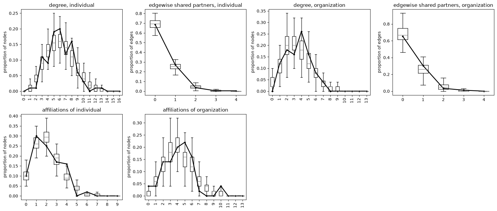
The model reproduces the degrees and shared partners within both levels. The numbers of affiliations are close, with a few more individuals with four and organizations with ten than the simulated networks usually have.
Estimating the decays#
MPNet fixes the weights of its alternating configurations; with
fixed=FALSE, ergmx estimates the decay along with the coefficients, as
ergm’s curved terms, from the start decay (by default log 2):
ergmx.ergm(network, "... + atxax('level', fixed=FALSE) + axs1b('level', fixed=FALSE)")
The statistics are the counts of the histogram each term weights (for
atxax, the A-ties with 1, 2… shared B partners), and the parameters the
coefficient and its decay, ATXAX.level and ATXAX.level.decay. A decay
is only identified if the network has a spread of those counts: in
linked_sim, few ties share more than one partner, and the decays are not.
Terms with two alternating parts (aaaxs, abaxs, asaxasb and the
directed ainasxainbs…) need a fixed decay.
Directed multilevel networks#
In a directed network, the ties within each level are arcs (advice among
researchers, partnerships from one laboratory to another), and the
affiliations are the arcs from the vertices of level A to those of level B
(A and B are the attribute’s values in sorted order, or levels=(A, B)).
The dyads from B to A carry no affiliation: fix them with blocks(), whose
second mixing type in a directed network is from the second level to the
first. S() with two sets takes the arcs from the first set to the second,
as in ergm. MPNet’s directed configurations then distinguish incoming and
outgoing ties, arcs and reciprocated pairs:
model = ergmx.ergm(
    network,
    "S(~edges + mutual, ~level == 'A') + S(~edges + mutual, ~level == 'B') "
    "+ S(~edges, (level == 'A') ~ (level == 'B')) "
    "+ in2starax('level') + txaxarc('level') + txbxreciprocity('level') + c4axbentrainment('level')",
    constraints="blocks('level', levels2=2)",
)
c4axbentrainment counts the four-cycles where an A-arc and a B-arc go
the same way between affiliated vertices (if laboratory u advises v, the
researchers of u advise those of v); c4axbexchange those where they go
opposite ways. The term reference
lists them all.
The tools below model the same undirected network by kinds of tie.
Densities by kind of tie#
nodemix('level', levels2=TRUE) has one statistic per mixing type, so
without an edges term each coefficient is the log-odds of a tie of that
kind:
densities = ergmx.ergm(linked, "nodemix('level', levels2=TRUE)")
densities.summary()
Maximum Likelihood Results:

                                      Estimate  Std. Error  MCMC %  z value  Pr(>|z|)
mix.level.individual.individual        -2.7267      0.0592       0  -46.059    <1e-04 ***
mix.level.individual.organization      -3.1422      0.0710       0  -44.263    <1e-04 ***
mix.level.organization.organization    -2.5466      0.1101       0  -23.136    <1e-04 ***
---
Signif. codes:  0 '***' 0.001 '**' 0.01 '*' 0.05 '.' 0.1 ' ' 1

Log-likelihood: -2323.5528   AIC: 4653.1055   BIC: 4675.0698
Affiliation ties are rarer, relative to the number of pairs, than ties within either level: about 4% of individual–organization pairs are tied, against 6% of pairs of individuals and 7% of pairs of organizations.
Closure within levels#
Do ties within a level close triangles? F(~gwesp(0.5, fixed=TRUE), ~nodematch('level')) computes gwesp on the network of the ties within
levels only:
closure = ergmx.ergm(
    linked,
    "nodemix('level', levels2=TRUE) + F(~gwesp(0.5, fixed=TRUE), ~nodematch('level'))",
    seed=1,
)
closure.summary()
Monte Carlo Maximum Likelihood Results:

                                        Estimate  Std. Error  MCMC %  z value  Pr(>|z|)
mix.level.individual.individual          -2.7639      0.0816       0  -33.883    <1e-04 ***
mix.level.individual.organization        -3.1434      0.0727       0  -43.262    <1e-04 ***
mix.level.organization.organization      -2.5769      0.1151       0  -22.387    <1e-04 ***
F(nodematch("level"))~gwesp.fixed.0.5     0.0415      0.0596       0    0.696   0.48652
---
Signif. codes:  0 '***' 0.001 '**' 0.01 '*' 0.05 '.' 0.1 ' ' 1

Log-likelihood: -2323.3112 (MC SE 0.010)   AIC: 4654.6225   BIC: 4683.9082
Converged after 3 iterations (4 chains, 1024 samples).
ergmx.compare(densities, closure)
Model comparison:

      df        log-likelihood         AIC         BIC     dAIC   LR chi2   df  Pr(>chi2)
  1    3             -2323.553     4653.11     4675.07     0.00
  2    4     -2323.311 (0.010)     4654.62     4683.91     1.52      0.48    1      0.487

  1: nodemix('level', levels2=True)
  2: nodemix('level', levels2=True) + F(gwesp(0.5, fixed=True), nodematch('level'))

Log-likelihoods of dyad-dependent models are Monte Carlo estimates (standard errors in parentheses).
Not in this simulated network: the coefficient is close to 0, and the comparison prefers the model without it.
The filter is any dyad-independent term with one statistic; a tie passes if
adding it would change that statistic. ~!nodematch('level') keeps the
other ties, here the affiliations.
Given the affiliations#
To model the ties within levels taking the affiliations as given, fix the
individual–organization dyads with blocks. Mixing types are numbered as
nodemix orders them: (individual, individual), (individual, organization),
(organization, organization), so the affiliations are type 2:
within = ergmx.ergm(
    linked,
    "nodemix('level', levels2=c(1, 3)) + F(~gwesp(0.5, fixed=TRUE), ~nodematch('level'))",
    constraints="blocks('level', levels2=2)",
    seed=1,
)
within.summary()
Monte Carlo Maximum Likelihood Results:

                                        Estimate  Std. Error  MCMC %  z value  Pr(>|z|)
mix.level.individual.individual          -2.7667      0.0825       0  -33.545    <1e-04 ***
mix.level.organization.organization      -2.5781      0.1149       0  -22.444    <1e-04 ***
F(nodematch("level"))~gwesp.fixed.0.5     0.0414      0.0601       0    0.688   0.49156
---
Signif. codes:  0 '***' 0.001 '**' 0.01 '*' 0.05 '.' 0.1 ' ' 1

Log-likelihood: -1461.4597 (MC SE 0.009)   AIC: 2928.9193   BIC: 2949.1041
Constraints: blocks('level', levels2=2).
Converged after 3 iterations (4 chains, 1024 samples).
blocks is dyad-independent, so the log-likelihood is still absolute, over
the free dyads, and BIC counts only those.
Fixed coefficients#
offset() fixes a coefficient rather than estimating it, for example to
compare networks of different sizes with a density adjusted for the
number of vertices (Krivitsky, Handcock and Morris 2011), or to forbid a
kind of tie with a coefficient of -inf:
# The same network without ties between organizations.
organizations = set(linked.vs.select(level="organization").indices)
without = linked.copy()
without.delete_edges([e for e in without.es if {e.source, e.target} <= organizations])

forbidden = ergmx.ergm(
    without,
    "nodemix('level', levels2=c(1, 2)) + offset(nodemix('level', levels2=3))",
    offset_coef=[float("-inf")],
)
forbidden.summary()
Maximum Likelihood Results:

                                              Estimate  Std. Error  MCMC %  z value  Pr(>|z|)
mix.level.individual.individual                -2.7267      0.0592       0  -46.059    <1e-04 ***
mix.level.individual.organization              -3.1422      0.0710       0  -44.263    <1e-04 ***
offset(mix.level.organization.organization)       -inf                                         (offset)
---
Signif. codes:  0 '***' 0.001 '**' 0.01 '*' 0.05 '.' 0.1 ' ' 1

Log-likelihood: -2004.5038   AIC: 4013.0076   BIC: 4027.4182
With the -inf offset, ties between organizations are impossible: the
model is fitted on the other dyads, and its simulated networks never have
them.